Maps are great for visualizing dry data.

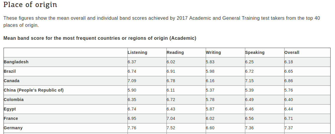
In this series of posts, I’ll demonstrate how to scrape websites in order to turn this:

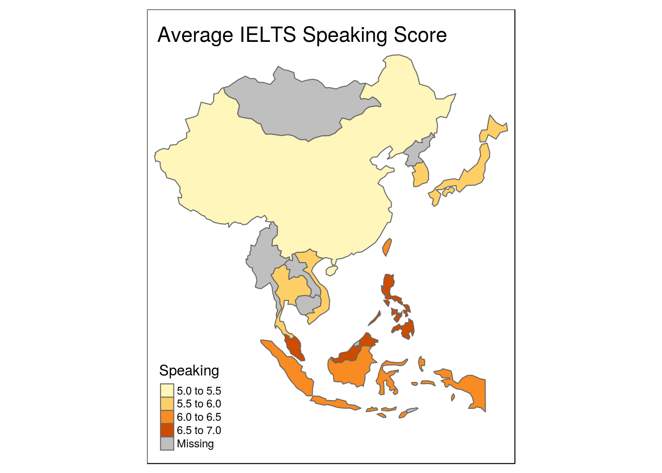
into this:

Today, I want to focus on scraping the requisite data for making the map above. Now I could just highlight the table, and then copy and paste it into a spreadsheet, but for really big tables that are spread over multiple pages, we’re going to want to do something that is more reproducible.

Step 1: Acquire Data from IELTS.org

First, we’ll load the necessary packages:

library(tidyverse)   #For cleaning
library(spData)      #For geom locations
library(rvest)       #For scraping sites

Now we need to load the website we want to scrape.

ielts.org <- read_html("https://www.ielts.org/teaching-and-research/test-taker-performance")

Next, we need to look at how the data is organized on the page were going to scrape. To do so, right click on the table of interest and select “inspect”.

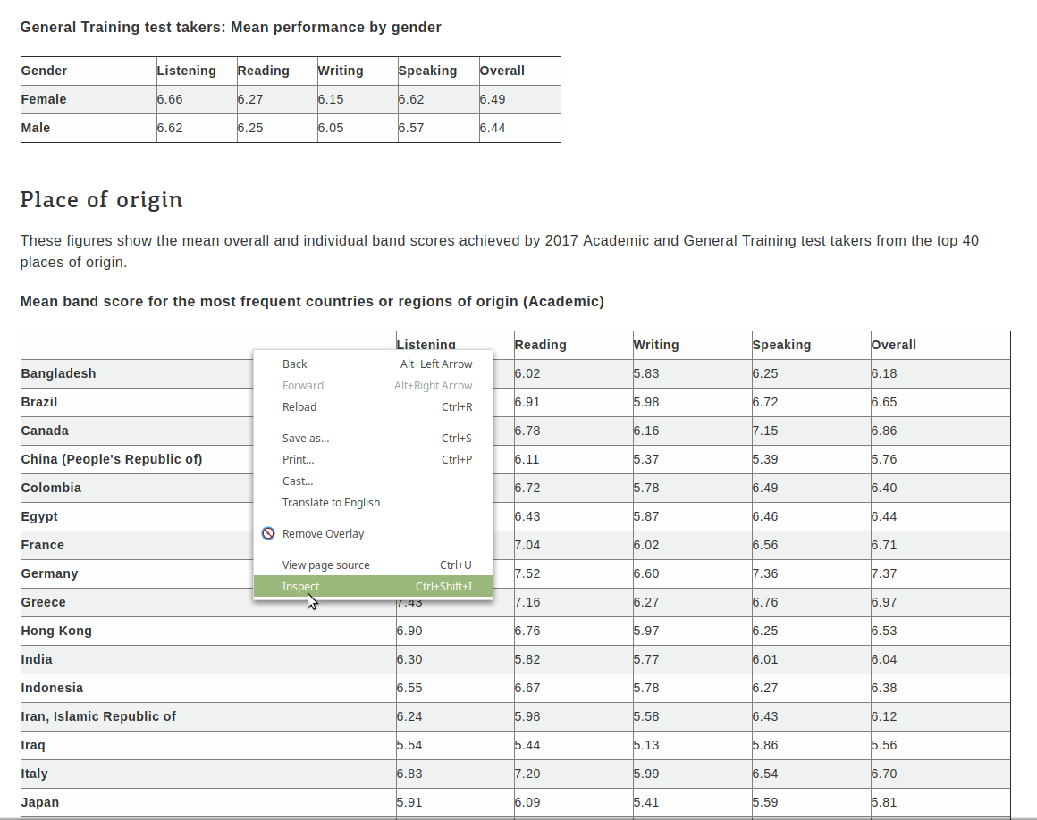
By using the inspection tool, we can find the specific table we want and scrape the data from there.

How do we do that?

1. Mouse over the elements until the desired table is highlighted
2. Right click on the element
3. Highlight “copy”
4. Select “Copy XPath” (see image below)

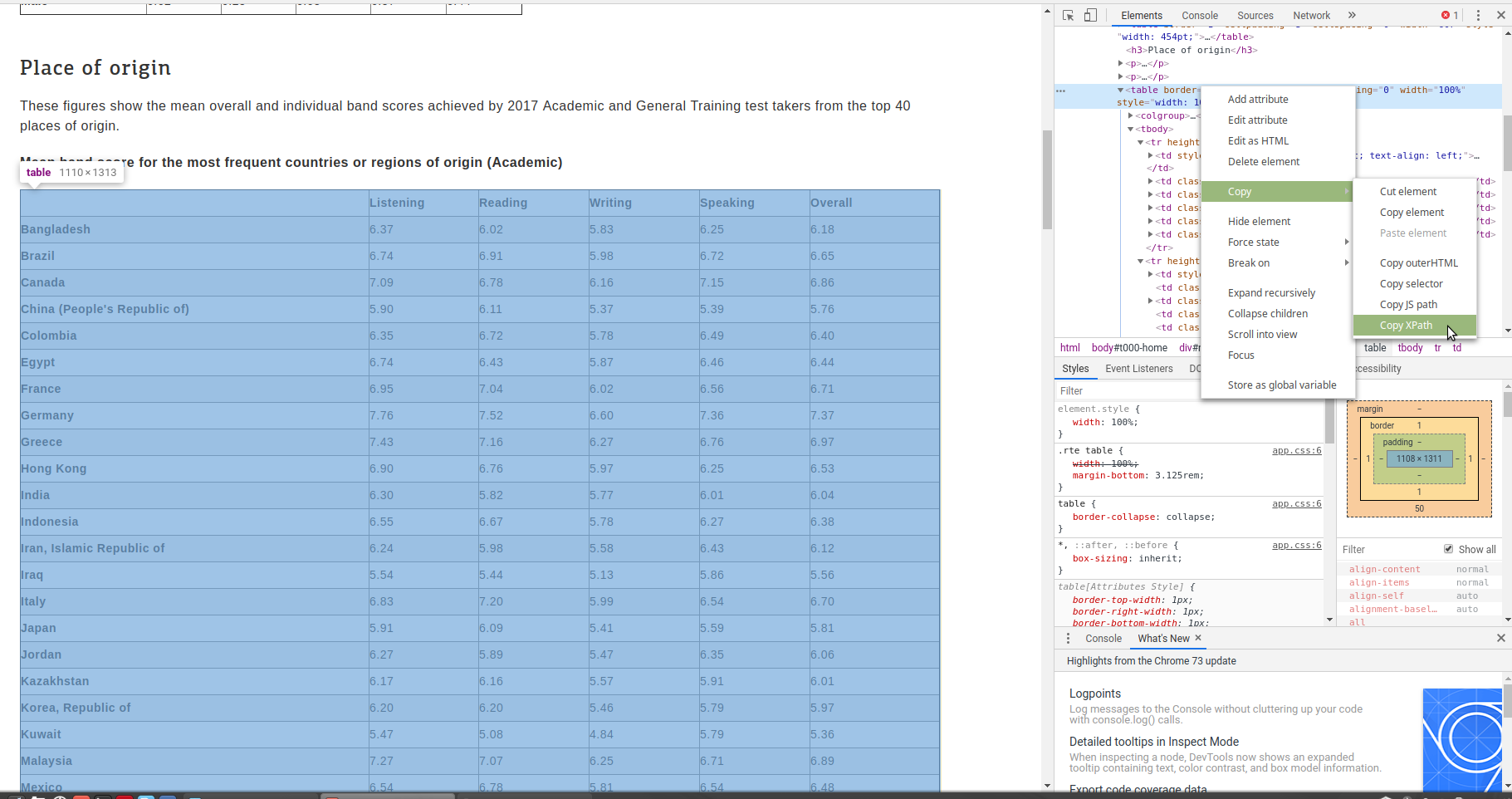
We’ve now loaded the website and identified the key information for extracting the table. All we have to do now is to pull the table from the website using some dplyr and rvest tools.

ielts.org %>% 
  html_node(xpath = '//*[@id="main"]/div/div/div[2]/table[3]') %>% 
  html_table(header = TRUE) -> scores_by_country

Translating the code above into English, we could say:

1. Select ielts.org and then
2. Select the specified element and then
3. Render it as a table (with headers) and save it as “scores_by_country”

Step 2: Acquiring Geographical Data

Getting the IELTS data was a little tricky. Getting our geographical data is much more straightforward: we take it directly from spData::world.

glimpse(world)

## Observations: 177
## Variables: 11
## $ iso_a2    <chr> "FJ", "TZ", "EH", "CA", "US", "KZ", "UZ", "PG", "ID", …
## $ name_long <chr> "Fiji", "Tanzania", "Western Sahara", "Canada", "Unite…
## $ continent <chr> "Oceania", "Africa", "Africa", "North America", "North…
## $ region_un <chr> "Oceania", "Africa", "Africa", "Americas", "Americas",…
## $ subregion <chr> "Melanesia", "Eastern Africa", "Northern Africa", "Nor…
## $ type      <chr> "Sovereign country", "Sovereign country", "Indetermina…
## $ area_km2  <dbl> 19289.97, 932745.79, 96270.60, 10036042.98, 9510743.74…
## $ pop       <dbl> 885806, 52234869, NA, 35535348, 318622525, 17288285, 3…
## $ lifeExp   <dbl> 69.96000, 64.16300, NA, 81.95305, 78.84146, 71.62000, …
## $ gdpPercap <dbl> 8222.2538, 2402.0994, NA, 43079.1425, 51921.9846, 2358…
## $ geom      <list> [<180.00000, 180.00000, 179.36414, 178.72506, 178.596…

Looking at the output, three variables are key for our task:

1. “name_long”: serves as the index to merge our data frames (more on that later).
2. “subregion”: provides the criteria for quickly filtering relevant countries.
3. “geom”: provides coordinates for making maps.

Step 3: Combining Dataframes

If we try to add our IELTS data to spData::world, it won’t work because the names of the countries do not perfectly align.

Therefore, to make life easy, we can change the country names in our IELTS data so that they match the default R data:

scores_by_country[scores_by_country == "Korea, Republic of"] <- "Republic of Korea"
scores_by_country[scores_by_country == "China (People's Republic of)"] <- "China"
scores_by_country[scores_by_country == "Taiwan, China"] <- "Taiwan"

What does the code above do? Essentially, it finds the value equal to “x” and replaces it with “y” or, in our case, find “Korea, Republic of” and replace it with “Republic of Korea.”

Next we can combine the two tables. Unfortunately, our country name column in “scores_by_country” is blank making it challenging to merge the two data frames.

So, first, we give that column the same name as spData::world which is “names_long”.

names(scores_by_country)[1] <- "name_long"

The code above means “Change the name of the first column of the data frame ‘scores_by_country’ to ‘name_long’“.

Now that both data frames have a column with the same name, we can merge them based on that shared column.

merge(x = world, y = scores_by_country, by = "name_long", all.x = TRUE)  -> scores_and_geoms

Again, walking through the code, we are telling R to combine the “world” and “scores_by_country” data frames based on a common column, “name_long”. Furthermore, we told it to keep all observations from world (hence all.x = TRUE) and to save this new data frame as scores_and_geoms.

Why didn’t we keep all scores_by_country and instead of world?

The focus of my analysis is on countries where I have the IELTS data but we won’t be able to meaningful maps unless we have all the geoms.

Now we have everything we need to make our maps which we’ll do in the next post.

Happy Coding!

#Full Code

#Load Libraries
library(tidyverse)   #For cleaning
library(spData)      #For geom locations
library(rvest)       #For scraping sites

#Read in IELTS.org
ielts.org <- read_html("https://www.ielts.org/teaching-and-research/test-taker-performance")

#Scrape IELTS.org
ielts.org %>% 
  html_node(xpath = '//*[@id="main"]/div/div/div[2]/table[3]') %>% 
  html_table(header = TRUE) -> scores_by_country

#Change country names
scores_by_country[scores_by_country == "Korea, Republic of"] <- "Republic of Korea"
scores_by_country[scores_by_country == "China (People's Republic of)"] <- "China"
scores_by_country[scores_by_country == "Taiwan, China"] <- "Taiwan"

#Assign a name to the country name
names(scores_by_country)[1] <- "name_long"

#Combine the two tables
merge(x = world, y = scores_by_country, by = "name_long", all.x = TRUE)  -> scores_and_geoms